Brief Syllabus:

Introduction: Governing equations for fluid flow and heat transfer, classifications of PDE, finite difference formulation, various aspects of finite difference equation, error and stability analysis, dissipation and dispersion errors, modified equations; Solutions of simultaneous equations: iterative and direct methods, TDMA, ADI; Elliptic PDE: One- and Twodimensional steady heat conduction and their solutions, extension to three-dimensional; Parabolic PDE: Unsteady heat conduction, explicit and implicit methods, solution of boundary layer equation, upwinding; Solution of incompressible N-S equation: Stream function and vorticity formulation, primitive variable methods: MAC and SIMPLE.

Objectives:

The primary objective of the course is to teach fundamentals of computational method for solving linear and non-linear partial differential equations (PDE). The course offers introductory concepts about solving PDE mainly in the finite difference (FD) framework though some amount of finite volume (FV) concept has also been introduced.

Prerequisites:

Knowledge of undergraduate heat transfer and fluid mechanics.

Course content:

Lecture-wise break-up (lecture duration: 50 minutes)

Suggested reference books:

• Computational Fluid Flow and Heat Transfer, Second Editionby K. Muralidhar, T. Sundararajan(Narosa), 2011.

• Computer Simulation of Flow and Heat Transfer by P. S. Ghoshdastidar (4th Edition, Tata McGraw-Hill), 1998.

• Numerical Computation of Internal and External Flows by Hirch C., Elesvier 2007.

Suggested reference books:

• Numerical Heat Transfer and Fluid Flow by S. V. Patankar(Hemisphere Series on Computational Methods in Mechanics and Thermal Science)

• Essential Computational Fluid Dynamics by Zikanov.O., Wiley 2010.

• Computational Fluid Dynamics by Chung T. J., Cambridge University Press, 2003.

Updated Syallabus:

Introduction. Basic Considerations in Design. Modelling of Thermal Systems. Numerical Modelling and Simulation. Acceptable Design of a Thermal System: A Synthesis of Different Design Steps. Optmization. Special Topics.

Lecturewise Breakup (based on 75min per lecture)

Lec # 1: Introduction:  Definition of Engineering Design.  Design Vs. Analysis- Examples.  Engineering Design: Decisions in an Engineering Undertaking- A Flow
Chart.  

Lec # 2: Thermal Systems: Basic Characteristics.  Definitions of System, Subsystem, Component and Process.  Basic Considerations in Design: Formulation of the Design Problem-(i) Requirements: Illustration by Examples.  To be continued.

Lec # 3: Formulation of Design Problem (Contd): (ii) Specifications. (iii) Given Quantities.  (iii) Design Variables: Hardware and Operating Conditions.  (iv)  Constraints and Limitations.  Example Problem showing a design problem and how to come up with a problem statement: Air-conditioning of a house.

Lec # 4: Steps in Design Process: A Flow Chart.  Example: Design of a Simple Counterflow Heat Exchanger-Acceptable Designs and Optimal Design.  Example: Design of a Refrigerator: Acceptable Designs and Optimal Design.

Lec # 5: Example: Design of a Quenching System for Hardening of a Steel Piece: an Example illustrating main steps in the design of a thermal system.  Material Selection: Properties and Applications of Metals and Alloys, Ceramics, Polymers, Composite Materials.  To be continued. 

Lec # 6: Material Selection (Contd): Liquids and Gases.  Selection and Substitution of Materials: Criteria. Various Examples of Material Selection.  Modelling of Thermal Systems:  Importance of Modelling in Design.  Basic Features of Modelling. 

Lec # 7:  Types of Models.  Interaction between Models.  Other Classifications. 
Mathematical Modelling: Transient/Steady State: Time Scales: Response Time of the Material or Body; Characteristic Time of Variation of the Ambient or Operating Conditions.  To be continued.   

Lec # 8: Time Scales (Completed).  Spatial Dimensions: How to determine dimensionality?  Lumped Mass Approximation.  Simplification of Boundary Conditions.  Negligible Effects: When do we neglect a particular effect?  Idealizations.  

Lec # 9: Material Properties.  Conservation Laws.  Example Problem.

Lec #10: Example Problem.  Curve Fitting: Exact Fit and Best Fit:  Applications.  Exact Fit: (a) General form of a polynomial.  To be continued.   

Lec # 11: Exact Fit (Contd):(b) Newton’s Divided-Difference Interpolating Polynomial.  (c) Lagrange Interpolation.  

Lec # 12:  Numerical Interpolation with Splines.  Best Fit: Basic Considerations.  Method of Least Squares- (i) Linear Regression.  Concept of Correlation Coefficient.  

Lec #13: Best fit with a Polynomial.  Nonpolynomial form.  Linearisation: Exponential, Power law and other functions.  Function of two or more independent variables: Exact Fit: y = f(x1, x2)-demonstration of the method using a second order polynomial.  

Lec # 14: Best Fit: y = f(x1, x2)-demonstration of the method using multiple regression analysis.  Extension to function of more than two independent variables.  Polynomial regression.  Linearisation of non-linear functions.  Numerical Modelling and Simulation: General Features.  Accuracy.  Solution of Linear Simultaneous Algebraic Equations: Direct Methods: (1) Gaussian Elimination: Basic method.  Advantages and Disadvantages.  Zero pivot element: Swapping of rows.  Small Pivot element: Example Problem.  Swapping with row having maximum pivot element.  To be continued.   

Lec # 15: Ill-conditioned and Well-conditioned System: Example.  (2) Gauss-Jordon Elimination Method: Basic Method.  Example.  (3) Matrix Decomposition Method.   

Lec # 16: (d) Matrix Inversion Method: Use of Gauss-Jordon method for matrix inversion.  Iterative Methods: (a) Jacobi Method.  (b) Gauss-Seidel Iterative Method.  Scarborough Criterion for Convergence.     

Lec # 17: Relaxation Method: Successive Over-relaxation and Under-relaxation.  Concept of Relaxation Factor.  Optimum Relaxation Factor.  Finite-Difference Method: Derivation of Central, Forward and Backward difference expressions for yi/ and yi// using Taylor series approach.  Concept of truncation error.  Finite-difference expressions of higher order accuracy.  

Lec # 18: Applications of finite-difference to Conduction Heat Transfer Problems: Steady 1 D heat transfer from a rectangular fin: Problem statement. Governing Differential Equation.  Non-dimensionalisation of GDE and B.C’s.  Discretization.  Image Point Technique: Handling of non-Dirichlet boundary conditions.  Matrix equations for 4 grid points at which temperatures are calculated.  Tri-diagonal coefficient matrix (TDM).  Tri-diagonal matrix algorithm (TDMA) or Thomas algorithm. 
Comparison of the numerical solution with analytical solution of the fin problem.  Numerical errors and accuracy: Round-off error, Truncation error and Total error.  Minimum total error.  Grid Independence Test. 

Lec # 19: 1D Fin with Convective Tip: Handling of tip boundary condition using image point technique.  2D Steady State Heat Conduction in a heat generating square block: Governing equation and boundary conditions.  Non-dimensionalization.  Discretization.  Handling of Corner Points.  Matrix equations for 4 x 4 grid points.  Advantage of having a banded coefficient matrix. Method of Solution: Choice between G-E and G-S.  Justification for using G-S.  Line-by-Line method.  3D Problems: Handling of corner and edge points.  

Lec #20: 1D Transient Heat Conduction in a Plane Wall: Governing equation, initial and boundary conditions.  Non-dimensionalization.  Explicit or Euler Scheme: Basis.  Finitedifference expressions for the case of four grid points.  Crank-Nicolson and Pure Implicit Schemes.     

Lec # 21: Definition of Stability.  von Neumann Stability Analysis for each scheme.   

Lec # 22: 2D Transient Conduction Problems: Applications of Euler, Pure Implicit, Crank-Nicolson and Alternating Direction Implicit (ADI) Method.  1D Transient Heat Conduction in Composite Media: Handling of the Interface by Taylor Series Approach.  
 
Lec # 23: Problems in Cylindrical Geometry: (a) Axisymmetric Problems (b) NonAxisymmetric Problems.  

Lec # 24: Non-linear GDE: Variable Thermal Conductivity.  Non-linear Boundary Condition: Radiation boundary Condition.  

Lec # 25: Numerical Model for a System: Isolating System parts.  Mathematical
Modelling.  Numerical Modelling.  Merging of Different Models.  System Simulation.  Importance of Simulation: Evaluation of design.  Off-design condition.  Optimization.  Improving or modifying existing systems.  Sensitivity tests.  Acceptable Design of a Thermal System:  Steps leading to acceptable design.     

Lec # 26:  Commonly used methods for obtaining an initial design.  Example Problem: Initial design of a Refrigerator.   

Lec # 27: Example Problem (Acceptable design not based on initial design): Design of a Solar Energy driven Water Heating System.  Iterative Redesign Procedure.  Example Problem: Design of Cooling of an Electronic Equipment:  Statement of the Problem.  To be continued.    
 
Lec # 28 Example Problem (Completed).  Heat Exchanger Design Problem: Given quantities, Requirements, Constraints, Design variables and Operating Conditions of a typical heat exchanger design problem.  

Lec # 29: Example Problem: Design of a Counterflow Double-Pipe Heat Exchanger: Statement of the Problem.  

Lec # 30: Problem Formulation for Optimization: Optimization in Design.  Basic Concepts: Objective Function.  Constraints: Equality Constraints and Inequality Constraints.  Conversion of Inequality Constraints to Equality Constraints by the use of
Slack Variables.  Steps involved in the formulation of an optimization problem.  List of Important Optimization Methods.  Calculus Methods: Basic Concepts. Maxima, Minima and saddle point for one variable and two variable problems.  Optimization involving objective function having more than two variables: Lagrange Multiplier Technique: Basic Method of Lagrange Multipliers for Constrained Optimization.  The Concept of Gradient Vector.  Lagrange Multiplier Equations.  

Lec # 31: Visualization of Lagrange Multiplier Method in Two Dimensions.  Unconstrained Optimization: Application of Lagrange Multiplier Method when there is no constraint.   Example Problems  (Conversion of a Constrained Optimization Problem into an Unconstrained Optimization Problem).

Lec # 32: Example Problem: Solution by Lagrange Multiplier Method for Constrained Optimization.  Sensitivity Coefficients.  Search Methods: Single Variable Problems: Uniform Exhaustive Search Method: Basic Concepts.  Expression for the Final Interval of Uncertainty.  Unimodal Functions: Examples of Continuous, Non-differentiable and Discontinuous Functions.  Use of Search Methods for Optimizing Non-Unimodal Functions.

Lec # 33: Eliminating a section based on two tests.  Dichotomous Search: The basic method.  The expression for the Final Interval of Uncertainty.  Fibonacci Search: Fibonacci Series.  The Steps in a Fibonacci Search.  Example Problem: Demonstration of the application of Fibonacci Search method to obtain the maxima of a function. Comparison of Effectiveness of Three Search Methods in terms of Reduction Ratio (RR).  

Lec # 34: Multivariable, Unconstrained Optimization: (a) Lattice Search; (b) Univariate Search.  Example Problem (Demonstration of Univariate Search for a Two-variable Problem). 

Lec # 35: (c) Steepest Ascent/Descent Method: Basis.  Basic Approach.  Algorithm.  Example Problem (Demonstration of Steepest Ascent/Descent Method for a Twovariable Problem).  

Lec # 36: Constrained Optimization: Penalty Function Method: Introduction.  Solution
Methodology.  Example Problem (Demonstration of Penalty Function Method for a TwoVariable Problem).  Geometric Programming: Introduction.  Form of Objective Function and Constraints.  Degree of Difficulty.  Solution Methodology for Single Variable Unconstrained Optimization Problem.  

Lec # 37: Mathematical Proof of Geometric Programming for Single Variable Unconstrained Optimization (with zero degree of difficulty).  Example Problem.  Example of a Difficult Expression of y* (containing a negative number raised to a negative non-integer): How to get around the problem? 

Lec # 38: Unconstrained, Multivariable Optimization (with Zero Degree of Difficulty): Methodology.  Example Problem.  Constrained, Multivariable Optimization (with Zero Degree of Difficulty): Methodology.  Example Problem.

Lec #39: Genetic Algorithm: Fundamentals.

Lec # 40-41: Special Topics (Suggested): 1. Optimization of Performance of a Power Cycle based on Exergy Analysis.  2.  Any other topic of the instructor’s choice.      

Textbooks:

1. Jaluria, Yogesh, 1998, Design and Optimization of Thermal Systems, McGrawHill, New York.

2. Deb, Kalyanmoy, 2006, Optimization for Engineering Design, Prentice-Hall, New Delhi.

Brief Syllabus:

Introduction, Details of an experimental setup, Static versus dynamic calibration, Design of experiments. Uncertainty analysis, Central limit theorem, Normal and Student’s-t distribution, Data outlier detection, Error propagation. Temporal response of probes and transducers, Measurement system model, zeroth, first, and second order systems, Probes and transducers, pressure transducers, pitot static tube, 5-hole probe, Hotwire anemometer, Laser Doppler velocimetry, Particle image velocimetry, Thermocouples, RTD, Thermister, Infrared thermography, Heat flux measurement, Interferometry, Schlieren and shadowgraph techniques, Holography, Measurements based on light scattering, Absorption spectroscopy, Mie scattering, Rayleigh, Raman and other scattering methods, Data acquisition systems, Analog to digital converter, Resolution, Quantization error, Signal connections, Signal conditioning, Digital signal and image processing, Review of numerical techniques, interpolation; curve fitting (regression), integration, differentiation, root finding, Solving a system of linear algebraic equations, Treatment of periodic data, Fourier analysis, FFT algorithm, Inverse FFT, Nyquist criterion, Numerical aspects of FFT, probability density function, auto- and cross-correlations, Optical tomography, ART family of algorithms Inverse techniques.

Lecture-wise breakup

 I: Introduction: Experiments versus simulation, Experiments versus measurements, Why conduct experiments, Details of an experimental setup, Principles of similarity; Global versus local measurements; Static versus dynamic calibration. (2 lectures)

 II: Design of experimen: issues related to probe selection, factorial design, design of experiments based on sensitivity function and uncertainty analysis. Examples related to (a) determining the duration of the experiment and (b) choosing between steady state and transient techniques. Forward versus inverse measurements, Examples related to wake survey, drag coefficient, and heat transfer coefficient. (2 lectures)

 III: Uncertainty analysis Nomenclature: precision versus accuracy, measurement errors, sampling, A/D conversion, attenuation, phase lag, signal-to-noise ratio, calibration. scatter, central limit theorem, 95% confidence interval, normal and Student’s-t distribution, data outlier detection, uncertainty, combining elemental errors, error propagation. (4 lectures)

 IV: Temporal response of probes and transducers: measurement system model, system response, amplitude response, frequency response, zeroth, first, and second order systems; examples of thermocouple response and U-tube manometer. Probe compensation in the frequency domain. (4 lectures)

 V: Probes and transducers: Pressure - pressure transducers; noise measurement
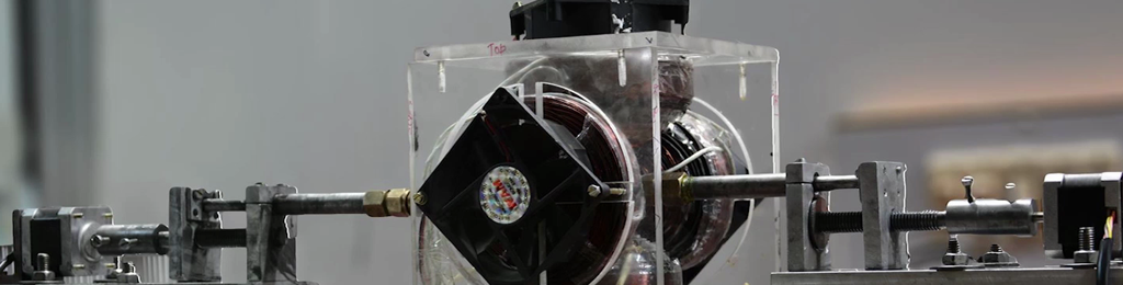
Velocity - pitot static tube (low as well as high speeds), 5-hole probe, Hotwire anemometer, CCA, CTA, Laser Doppler velocimetry, Particle image velocimetry.  Temperature measurement: thermocouples, RTD, thermister, infrared thermography, Heat flux measurement,  (10 lectures)

 VI: Refractive index based optical measurement techniques:Introduction to lasers, interference, interferometry, fringe analysis; Schlieren and shadowgraph techniques; Image analysis using ray tracing technique; Holography (5 lectures)

 VII: Measurements based on light scattering:absorption spectroscopy, shadow formation, Mie scattering, Rayleigh, Raman and other scattering methods. (3 lectures)

 VIII: Data acquisition systems:analog input-output communication, analog to digital converter, static and dynamic characteristic of signals, Bits, Transmitting digital numbers, resolution, quantization error, signal connections, single and differential connections, signal conditioning. (3 lectures)

 IX: Digital signal and image processing:Digital signal processing compared with digital image processing signal conditioning. (6 lectures)

• Review of numerical techniques: interpolation; curve fitting (regression), integration, differentiation, root finding, solving a system of linear algebraic equations. 

• Treatment of periodic data; Fourier analysis, FFT algorithm; Inverse FT; Nyquist criterion. Numerical aspects of FFT; probability density function; auto- and crosscorrelations

• Optical tomography, ART family of algorithms 
  Inverse techniques: Determination of thermophysical properties using inverse techniques.

Demonstration experiments:

Several demonstration experiments will be used for explaining the implementation details of several experimental techniques. Some examples are:

• Determination of wall shear stress of flat plate boundary layer; 

• Determination of drag coefficient of circular cylinder in cross-flow;

• time-averaged and rms fluctuations in a turbulent mixing layer; (d) viscosity measurement;

• Determination of average Nusselt number of a circular cylinder in cross flow

• Visualization using Interferometry, schlieren, shadowgraph, digital holography and infrared thermography

• Velocity distribution around cylinder using PIV

References:

1. C. Tropea, A.L. Yarin, and J.F. Foss, Editors, Springer Handbook of Experimental Fluid Mechanics, 2007.

2. T.G. Beckwith and N.L. Buck, Mechanical Measurements, Addison-Wesley, MA (USA), 1969.

3. H.W. Coleman and W.G. Steele Jr., Experiments and Uncertainty Analysis for Engineers, Wiley & Sons, New York, 1989.

4. E.O. Doeblin,  Measurement Systems, McGraw-Hill, New York, 1986.

5. R.J. Goldstein (Editor), Fluid Mechanics Measurements, Hemisphere Publishing Corporation, New York, 1983; second edition, 1996.

6. J. Hecht, The Laser Guidebook,  McGraw-Hill, New York, 1986.

7. B.E. Jones, Instrumentation Measurement and Feedback, Tata McGraw-Hill, New Delhi, 2000.

8. M. Lehner and D. Mewes,  Applied Optical Measurements, Springer-Verlag, Berlin, (1999).

9. F. Mayinger, Editor, Optical Measurements: Techniques and Applications, SpringerVerlag, Berlin, 1994. 

10. D.C. Montgomery, Design and Analysis of Experiments, John Wiley, New York, 2001.

11. A.S. Morris, Principles of Measurement and Instrumentation, Prentice Hall of India, New Delhi, 1999.

12. F. Natterer, The Mathematics of Computerized Tomography, John Wiley & Sons, New York, 1986.

13. P.K. Rastogi, Ed., Photomechanics, Springer, Berlin, 2000.

14. M. Van Dyke, An Album of Fluid Motion, The Parabolic Press, California, 1982.